Time Series Analysis Part 4 – Multiple Linear Regression
Over the past 3 articles on time series we applied ARMA, ARIMA and SARIMA to time series examples and proceeded toward model selection via either AIC (Akaike Information Criterion) or MSE on unseen data. Here, we approach the same time series as found in Time Series Analysis Part 3 – Assessing Model Fit from a Linear Regression point of view.
Here is the same time series data as in Part 3:

This series contains 500 data points. We split this dataset into a test (first 400 data points) and train (final 100 data points):


We will need to transform the training data to a format a regression model can work on. First, let us start with a single lag 
The Linear Regression fit to this dataset looks like this:


It is clear that this model is missing quite a substantial set of predictors. In particular the trend. First, we need to add a ‘time’ predictor variable. This is where the trend component will come into play. The transformed dataset and the fit looks like this:

This is a little better than before. We can see that we have captured the trend as well as reduced the MSE on the test set from 39 to 22.56. To improve this model, we can observe that there is seasonality in the data. We did this in the previous 3 articles on time series by observing the ACF and found that the series as a seasonality of 20. We will introduce this into the model by way of transforming the dataset to include a seasonality component. The transformed dataset below introduces seasonality by taking modulo 20 of the time column (time % 20):
These extra seasonality predictors provide additional information to the Linear model so that an adjustment can be made to the average value reflecting the position of the datapoint in the seasonality. For example the coefficient of season_20 in the regression is 1.7. This means the average value (predicted using the trend and lag 1) is adjusted by 1.7 every 20 datapoints. The predictions on the test set now looks like this:

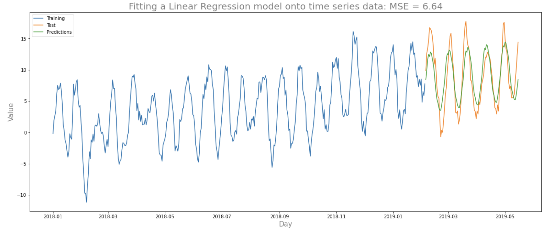
We observe 2 improvements to the fit on the test set: the predictions much better fit the test set thanks to the seasonality; the MSE has dropped greatly to 6.8. We can add more lags to improve the fit:


We have managed to reduce the MSE to 6.64 by including lags up to 4 and an MSE of 8.24 with lags up to 30. Note that the regression output shows that there are quite a few predictors that are not significant. We can tackle this using regularisation techniques to ensure we reduce the effects of overfitting the dataset. We won’t do this here as this would need the creation of a dev set for the hyper-parameter tuning. Another note here is that just because we attained a certain MSE on this test set doesn’t necessarily mean that the performance best represents performance on unseen data in general. To obtain a better representation of the MSE on unseen data we perform time series cross validation as seen in the previous article.
In Time Series Analysis Part 3 – Assessing Model Fit, the SARIMA(2, 0, 4, 3, 1, 1, 20, ‘c’) model attained an average MSE of 4.93 on a time series cross-validated dataset. For the model developed using Linear Regression here (with 30 lags), we attain an average MSE of 5.08. This is quite good.
For diagnostic purposes we can check the Q-Q plot for the residuals to make sure the residuals are roughly normally distributed:

We have seen that Multiple Linear regression can be applied to time series data with some good results. However, this was a toy example with us having full control over the generation of the time series data. A more representative test of differences in the performance of these approaches should be applied to real world time series data. Which brings us to the next article…