Time Series Analysis Part 3 – Assessing Model Fit

In Time Series Analysis Part 1 – Identifying Structure, we were introduced to the techniques used to identify the underlying time series structure. This naturally led to the desire to forecast once the most likely underlying structure was identified. In Time Series Analysis Part 2 – Forecasting, we were able to work this magic on a particular time series dataset while also tackling the seasonality component and arriving at a model we think best describes the data. We then went on to forecast using the discovered model. After overlaying the forecasted predictions onto the dataset, this is what it looked like:

In the previous posts, we identified the quality of the model through either the Akaike Information Criterion (AIC) or an F-Test while comparing nested models. Either approach can be used to determine the better model however AIC seems to be more popular.

In the fit shown above, we want to understand how well the model predicts unseen data. The final 100 data points of the 500 data point long time series shown was unseen to the model and left out as a Test Set. The Mean Squared Error (MSE) is a simple measure used to gain some insight into the quality of the predictions relative to the Test Set:

where is the number of data points, is the actual value of the observed time series value and is the prediction of that value. Sometimes the square root of this value (the RMSE) is used because it retains the original units of the dataset. The MSE of the above fit is:

or

On its own, this value doesn’t mean much. Only that on average we are about 3 units away from our predictions which, given that the data fluctuates across 20 units, sounds pretty good. The MSE is most meaningful and useful when comparing between different models for the purpose of assessing which predictive model to be used.

However, before we apply a bunch of other models and calculate their MSEs, notice in the time series above that while there is clear seasonality (a pattern of peaks and troughs), sometimes that pattern is violated. For example the peak before 2018-03 follows and uncharacteristically low trough. Similarly, the peak after 2018-11 is unusually high. It is clear that some randomness exists in the original time series data. Ideally, we want to identify the model that best deals with these cases that are uncharacteristic of the underlying data while minimising its impact on the quality of its predictions. Additionally, we do not want the model to be lucky that it was able to perform well because it was trained on a particular portion (the first 400) and predicted on another particular portion (the final 100) of the dataset.

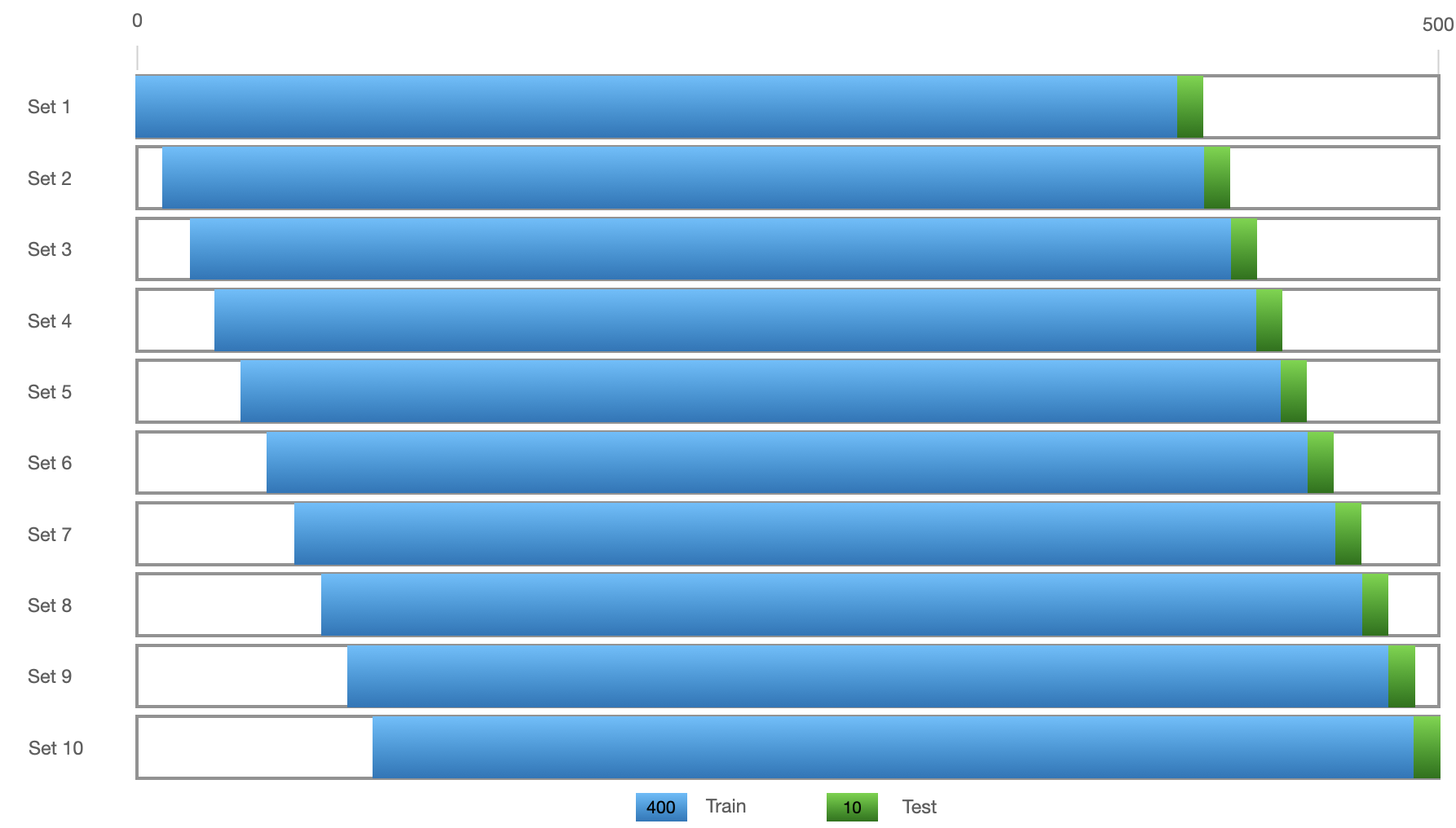
To get a better understanding of the performance on unseen data, we can create 10 train/test pairs as follows:

Performing 10 train-tests on the model shown at the beginning of the post gives an average MSE of:

Here, we have approached model selection in a different way to using AIC or performing F-Tests which were more relevant to regressions. This approach of using the MSE of predictions on unseen data can be applied regardless of the type of model we want to apply.

In the previous post, we performed a stepwise search to find the model that has the smallest AIC. This time we select the best model using the average MSE:

We have found 2 other models which perform better on unseen data than the model chosen using the AIC approach. By the way, these are all good fits, as can be seen by the overlayed predictions from these models below:

In the next post we will approach this problem by applying Multiple Linear Regression to this dataset by building up a feature list we believe should help explain some of the patterns seen in time series data.